Examples of using catLGM
These demos illustrate the use of catLGM.m function to solve variety of machine learning problems. The code used to generate these demos can be downloaded here.
To run these demos, change directory to catLGM/ and do addpath(genpath(pwd)).
Return to catLGM main pageContents
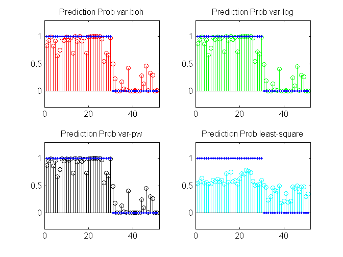
Binary Classification with Bayesian Logistic Regression
    clear all;
    setSeed(1)
    % generate data
    N = 5000; Ntrain = 4000;
    X = 2*rand(N, 2)-1;
    y = (sigmoid(X*[1; -1]))>0.5;
    y = ~y + 1; % Always specify binary data in [1 2] coding instead of [1 0]
    idx = randperm(N);
    ytrain = y(idx(1:Ntrain)); Xtrain = X(idx(1:Ntrain),:);
    ytest = y(idx(4950:end)); Xtest = X(idx(4950:end),:);
    ytest_bit = bsxfun(@eq, ytest, [1 2]);

    % specify model, algorithm and options
    model = 'bayesLogitReg';
    algos = {'var-boh','var-log','var-pw'};
    options = struct( 'maxItersInfer', 100, 'lowerBoundTolInfer', 0.001, 'displayInfer', 0);

    % Run each algorithm
    for i = 1:length(algos)
      % inference and prediction
      postDist{i} = catLGM('bayesLogitReg', 'infer', algos{i},  [Xtrain ytrain], options);
      pred(:,:,i) = catLGM('bayesLogitReg', 'predict', 'mc',  Xtest, [], postDist{i});

      % compute cross entropy error and store
      predErr(i) = -sum(sum(ytest_bit.*log2(pred(:,:,i)),2),1)/length(ytest);
      predProb(:,i) = pred(:,1,i);
      logLik(i) = postDist{i}.logLik;
      w(:,i) = postDist{i}.mean;
    end

    % least squares with (1,-1) encoding
    yc = -(2*ytrain-3); % change to (1,-1)
    w_ls = inv(Xtrain'*Xtrain)*Xtrain'*yc;
    w(:,end+1) = w_ls;
    p_ls = sigmoid(Xtest*w_ls);
    p_ls = [p_ls 1-p_ls];
    predErr(end+1) =-sum(sum(ytest_bit.*log2(p_ls),2),1)/length(ytest);
    predProb(:,end+1) = p_ls(:,1);
    algos{end+1} = 'least-square';
    logLik(end+1) = NaN;

    % display
    algos
    fprintf('Estimated Weights: \n '); w
    fprintf('Prediction error\n '); predErr
    fprintf('Training log-lik\n '); logLik

    % plot
    [tt1,idx] = sort(ytest);
    figure(1); clf;
    colors = {'r','g','k','c'};
    for i = 1:length(algos)
      subplot(2,2,i);
      stem(predProb(idx,i),'r', 'color', colors{i});
      hold on;
      plot(ytest_bit(idx,1),'.','linewidth',4);
      xlim([0 length(ytest)+1]); ylim([-0.3 1.3]);
      title(sprintf('Prediction Prob %s', algos{i}));
    end
algos =

    'var-boh'    'var-log'    'var-pw'    'least-square'

Estimated Weights:

w =

    9.4560   11.0330   11.2652    1.0153
   -9.4208  -11.0141  -11.2466   -0.9932

Prediction error

predErr =

    0.2089    0.1847    0.1812    0.7174

Training log-lik

logLik =

 -420.2152 -416.5018 -450.3729       NaN
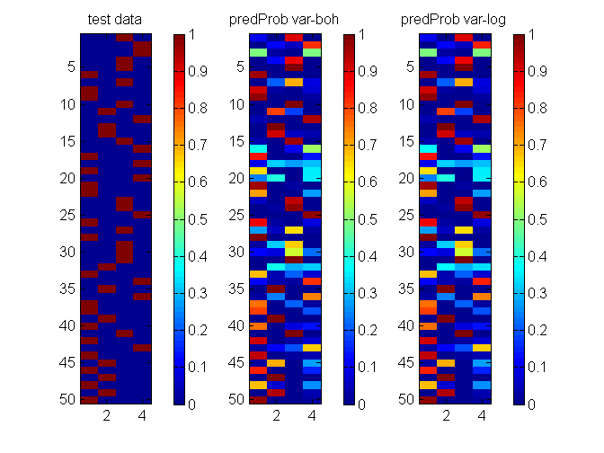
Multi-Class classification using Bayesian Multinomial-Logit Regression
    clear all;
    % generate data
    N = 1000; F = 5; nClass = 4;
    X = 2*rand(N, F)-1;
    beta = randn(nClass,F);
    eta = X*beta';
    lse = logsumexp(eta,2);
    prob = bsxfun(@minus, eta, lse);
    prob = exp(prob);
    [junk,y] = max(prob,[],2);
    Ntest = 50; Ntrain = ceil(0.8*N);
    idx = randperm(N);
    ytrain = y(idx(1:Ntrain));
    Xtrain = X(idx(1:Ntrain),:);
    ytest = y(idx(N-Ntest+1:end));
    Xtest = X(idx(N-Ntest+1:end),:);
    ytest_bit = bsxfun(@eq, ytest, [1:nClass]);

    % specify model, algorithm and options
    model = 'bayesMultiLogitReg';
    algos = {'var-boh','var-log'};
    options = struct('maxItersInfer', 1000, 'lowerBoundTolInfer', 1e-5, 'displayInfer', 0);

    % Run each algorithm
    for i = 1:length(algos)
      postDist{i} = catLGM(model, 'infer', algos{i},  [Xtrain ytrain], options);
      predProb(:,:,i) = catLGM(model, 'predict', 'mc',  Xtest, [], postDist{i});

      % compute cross entropy error and store
      predErr(i) = -sum(sum(ytest_bit.*log2(predProb(:,:,i)),2),1)/length(ytest);
      logLik(i) = postDist{i}.logLik;
      w(:,i) = postDist{i}.mean;
    end

    % display
    algos
    w
    predErr
    logLik

    % plot
    figure(1); clf;
    nr = 1; nc = size(predProb,3) + 1;
    subplot(nr,nc,1);
    imagesc(ytest_bit); colorbar; caxis([0 1]);
    title('test data');
    for i = 1:size(predProb,3)
      subplot(nr,nc,i+1);
      imagesc(predProb(:,:,i)); colorbar; caxis([0 1]);
      title(sprintf('predProb %s', algos{i}));
    end
algos =

    'var-boh'    'var-log'


w =

    5.2856    5.2865
   -0.5911   -0.5971
   -3.0405   -3.0356
   -1.1945   -1.1917
    0.5754    0.5728
   -4.4748   -4.5063
   -4.0890   -4.1053
   -2.2287   -2.2379
    1.0797    1.0892
   -0.9744   -0.9858
    3.9102    3.9116
   -7.2525   -7.2706
    0.3131    0.3162
   -3.6087   -3.6150
    2.1769    2.1784


predErr =

    0.3414    0.3413


logLik =

 -303.3138 -301.7505
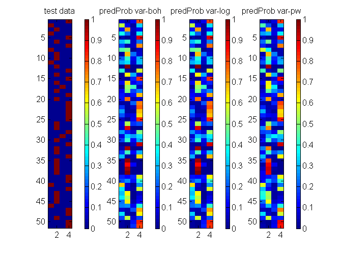
Multi-Class Gaussian Process Classification
    clear all;
    % generate data
    N = 1000; F = 2; nClass = 4;
    X = randn(N, F);
    beta = [0 0; 1 0; 0 1; -1 1];
    eta = X*beta';
    lse = logsumexp(eta,2);
    prob = bsxfun(@minus, eta, lse);
    prob = exp(prob);
    [junk,y] = max(prob,[],2);
    Ntrain = ceil(N*0.1);
    idx = randperm(N);
    ytrain = y(idx(1:Ntrain));
    Xtrain = X(idx(1:Ntrain),:);
    ytest = y(idx(950:end));
    Xtest = X(idx(950:end),:);
    ytest_bit = bsxfun(@eq, ytest, [1:nClass]);

    % mean and covariance functions and their hyper-parameters
    params.meanfunc = {@meanZero};
    params.covfunc = {@covSEiso};
    params.hyp.mean = [];
    params.hyp.cov = 1*ones(nClass-1,2);
    params.others.nClass = nClass;

    % Specify model and algorithm
    models = {'multiLogitGP', 'multiLogitGP', 'stickLogitGP'};
    algos = {'var-boh', 'var-log', 'var-pw'};
    options = struct('maxItersInfer', 1000, 'lowerBoundTolInfer', 1e-5, 'displayInfer', 0);

    % Run each algorithm
    for i = 1:length(algos)
      inferOut{i} = catLGM(models{i}, 'infer', algos{i}, [Xtrain ytrain], options, params);
      predProb(:,:,i) = catLGM(models{i}, 'predict', 'mc',  Xtest, [], inferOut{i});
      predErr(i) = computeCrossEntropy(predProb(:,:,i)', ytest, nClass);
      logLik(i) = inferOut{i}.logLik;
    end

    % display
    algos
    predErr
    logLik

    % plot
    figure(2); clf;
    nr = 1; nc = size(predProb,3) + 1;
    subplot(nr,nc,1);
    imagesc(ytest_bit); colorbar; caxis([0 1]);
    title('test data');
    for i = 1:size(predProb,3)
      subplot(nr,nc,i+1);
      imagesc(predProb(:,:,i)); colorbar; caxis([0 1]);
      title(sprintf('predProb %s', algos{i}));
    end
algos =

    'var-boh'    'var-log'    'var-pw'


predErr =

    0.6974    0.6864    0.7562


logLik =

  -82.1167  -75.2715  -75.8875
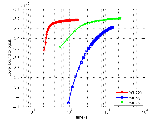
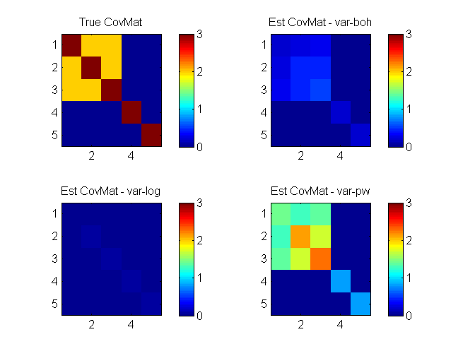
Binary Latent Gaussian Graphical Model
    clear all;
    % generate data
    D=5;
    mean_ = [2 1 0.5 0 0]';
    X1 = [1 1 1; 0 0 0]; X2 = [0 0; 0 1; 1 0; 1 1];
    X=[X1(repmat(1:2,4,1),:), repmat(X2,[2,1])];
    C=7*cov(X)+eye(D);
    covMat = C;
    S  = 100000;
    z  = mvnrnd(mean_,C,S);
    az = sigmoid(z')';
    Y = (az>rand(S,D))';

    % Always change binary data to [1 2] coding instead of [1 0]
    Y = ~Y + 1;

    % specify model, algos and options
    model = 'binaryLogitLGGM';
    algos = {'var-boh','var-log','var-pw'};
    options = struct('lowerBoundTolLearn', 0.01,'displayLearn',0);
    nIters = [200 50 50];

    % run each algorithm
    for i = 1:length(algos)
      options.maxItersLearn = nIters(i);
      out{i} = catLGM(model, 'learn', algos{i},  Y, options);
      mean_(:,i+1) = out{i}.params.mean;
      covMat(:,:,i+1) = out{i}.params.covMat;
    end

    % plot
    figure(1); clf;
    h(1) = semilogx(out{1}.time, out{1}.logLik, 'ro-', 'linewidth',2);
    hold on
    h(2) = semilogx(out{2}.time, out{2}.logLik, 'bs-', 'linewidth',2);
    h(3) = semilogx(out{3}.time, out{3}.logLik, 'gx-', 'linewidth',2);
    xlim([0.05 100]);
    grid on;
    legend(h, algos, 'location', 'southeast');
    xlabel('time (s)');
    ylabel('Lower bound to logLik');
    fprintf('Estimated mean\n');
    ['truth' algos]
    mean_
    figure(2); clf;
    nr = 2; nc = 2;
    for i = 1:size(mean_,2)
      subplot(nr,nc,i)
      imagesc(covMat(:,:,i)); colorbar; caxis([0 max(C(:))]);
      if i ~=1; title(sprintf('Est CovMat - %s', algos{i-1}));
      else title('True CovMat');
      end
    end
Estimated mean

ans =

    'truth'    'var-boh'    'var-log'    'var-pw'


mean_ =

    2.0000    1.3461    0.9507    1.6454
    1.0000    0.6766    0.5080    0.9178
    0.5000    0.3350    0.2318    0.4774
         0    0.0015   -0.0982   -0.0005
         0    0.0052   -0.0949    0.0035
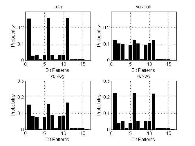
Categorical Factor Analysis
    clear all
    % D dimensions with M categories and N data points
    D = 2; M = 4;
    nC = M*ones(D,1);
    N = 10000;
    L = (M-1)*D;
    X = [eye(M-1) eye(M-1)];
    C = 20*cov(X) + eye(D*(M-1));
    covMat = C;
    mean_ = zeros(L,1);
    z = mvnrnd(mean_(:)', covMat, N);
    for d = 1:D
      idx = [1:M-1] + (d-1)*(M-1);
      eta_d = [z(:,idx)'; zeros(1,N)];
      lse = logsumexp(eta_d,1);
      prob = exp(bsxfun(@minus, eta_d, lse));
      [junk, Y(:,d)] = max(prob);
    end
    Y = Y';

    % compute true data distribution
    [Yt,I,J]  = unique(Y','rows');
    dist(1,:) = hist(J,1:size(Yt,1))/size(Y,2);

    % specify models, and corresponding algos and options
    models = {'multiLogitFA','multiLogitFA','stickLogitFA'};
    algos = {'var-boh','var-log','var-pw'};
    options = struct('lowerBoundTolLearn', 0.01,...
                     'displayLearn',0,...
                     'maxItersInfer',10,...
                     'maxItersLearn', 100,...
                     'latentDim', 2);

    % run algorithms
    for i = 1:length(algos)
      out{i} = catLGM(models{i}, 'learn', algos{i},  Y, options);
      mean_ = out{i}.params.mean;
      covMat = out{i}.params.covMat;
      W = out{i}.params.loadingMat;
      bias = out{i}.params.bias;
      [dist(i+1,:), Y1] = computeCatDist_mc(models{i}, mean_, covMat, W, bias, nC);
    end

    % plot
    figure(1);
    nr = 2; nc = 2;
    subplot(nr,nc,1)
    bh = bar(dist(1,:), 'facecolor', 'k', 'edgecolor', 'k');
    ylim([0 .30]); xlim([0 17]);
    grid on;
    hx = xlabel('Bit Patterns');
    hy = ylabel('Probability');
    ht = title('truth');
    for i = 2:length(algos)+1
      subplot(nr,nc,i)
      bh = bar(dist(i,:), 'facecolor', 'k', 'edgecolor', 'k');
      ylim([0 .3]); xlim([0 17]);
      grid on;
      hx = xlabel('Bit Patterns');
      hy = ylabel('Probability');
      ht = title(algos{i-1});
    end
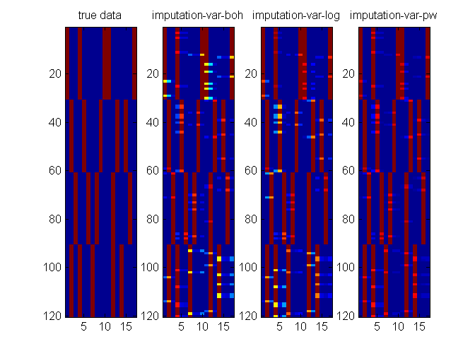
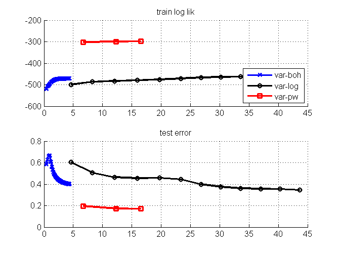
Missing data imputation
    clear all; close all;
    % genearate data
    Y = [ repmat([1; 1; 4; 1; 4], 1, 30)...
          repmat([2; 2; 3; 3; 2], 1, 30)...
          repmat([3; 3; 2; 2; 3], 1, 30)...
          repmat([2; 1; 1; 2; 1], 1, 30)];
    nC = [3; 3; 4; 3; 4];
    Ybitvec = encodeDataOneOfM(Y, nC, 'M');
    [D,N] = size(Y);

    % create one missing entry in part of the data
    d = unidrnd(D,1,N); % one missing dim in each data point
    ratio = 0.5; % ratio of missing data examples
    Ymiss = Y;
    nMiss = 0;
    for i = 1:size(Y,2)
      if rand <ratio
        Ymiss(d(:,i),i) = NaN;
        nMiss = nMiss + length(unique(d(:,i))); % #miss
      end
    end

    % specify models, algorithms, and options for imputation
    models = {'multiLogitFA', 'multiLogitFA', 'stickLogitFA'};
    algos = {'var-boh', 'var-log', 'var-pw'};
    colors = {'bx-','ko-','rs-'};
    nIters = [35 12 3];
    options = struct('maxItersLearn', 5,...
                     'lowerBoundTolLearn', 0.001,...
                     'displayLearn',0,...
                     'maxItersInfer',10,...
                     'maxItersMstep',5,...
                     'latentDim',5);

    % plot true data
    figure(2); clf;
    nr = 1; nc = length(algos)+1;
    subplot(nr,nc,1);
    imagesc(Ybitvec');
    title('true data');
    figure(1); clf;

    % data imputation
    for m = 1:length(algos)
      fprintf('EM for Parameter learning\n');
      params = [];
      initVec = [];
      algos{m}
      for iter = 1:nIters(m)
        % warm start from previous iterations of EM
        options.initVec = initVec;

        % learn model
        learnOut = catLGM(models{m}, 'learn', algos{m}, Ymiss, options, params);

        % read output
        params = learnOut.params; % learned parameter
        postDist = learnOut.postDist; % post Dist
        initVec = learnOut.ss.initVec; % for next iteration
        trLogLik(iter) = learnOut.logLik(end);
        tt(iter) = learnOut.time(end);

        % impute data
        pred = catLGM(models{m}, 'impute', 'mc', Ymiss, [], params, postDist);
        err(iter) = -sum(sum(Ybitvec.*log2(max(pred,eps))))/nMiss;

        % plot
        figure(1);
        subplot(2,1,1);
        hold on
        h1(m) = semilogx(cumsum(tt), trLogLik, colors{m}, 'linewidth',2);
        grid on;
        title('train log lik');
        subplot(2,1,2);
        hold on
        grid on;
        semilogx(cumsum(tt), err, colors{m}, 'linewidth',2);
        title('test error');
        drawnow;
        figure(2);
        subplot(nr,nc,m+1);
        imagesc(pred');
        title(sprintf('imputation-%s', algos{m}));
        drawnow;
      end
      clear err trLogLik tt;
    end

    figure(1); subplot(2,1,1);
    legend(h1, algos, 'location', 'southeast');
EM for Parameter learning

ans =

var-boh

EM for Parameter learning

ans =

var-log

EM for Parameter learning

ans =

var-pw